Data exploration calculus Capturing the essence of exploratory data scripting

Most real-world programming languages are too complex to be studied using formal methods. For this reason, academics often work with simple theoretical languages instead. The λ-calculus is a simple formal language that is often used for talking about functional languages, the π-calculus is a model of concurrent programming and there is an entire book, A Theory of Objects modelling various object-oriented systems.

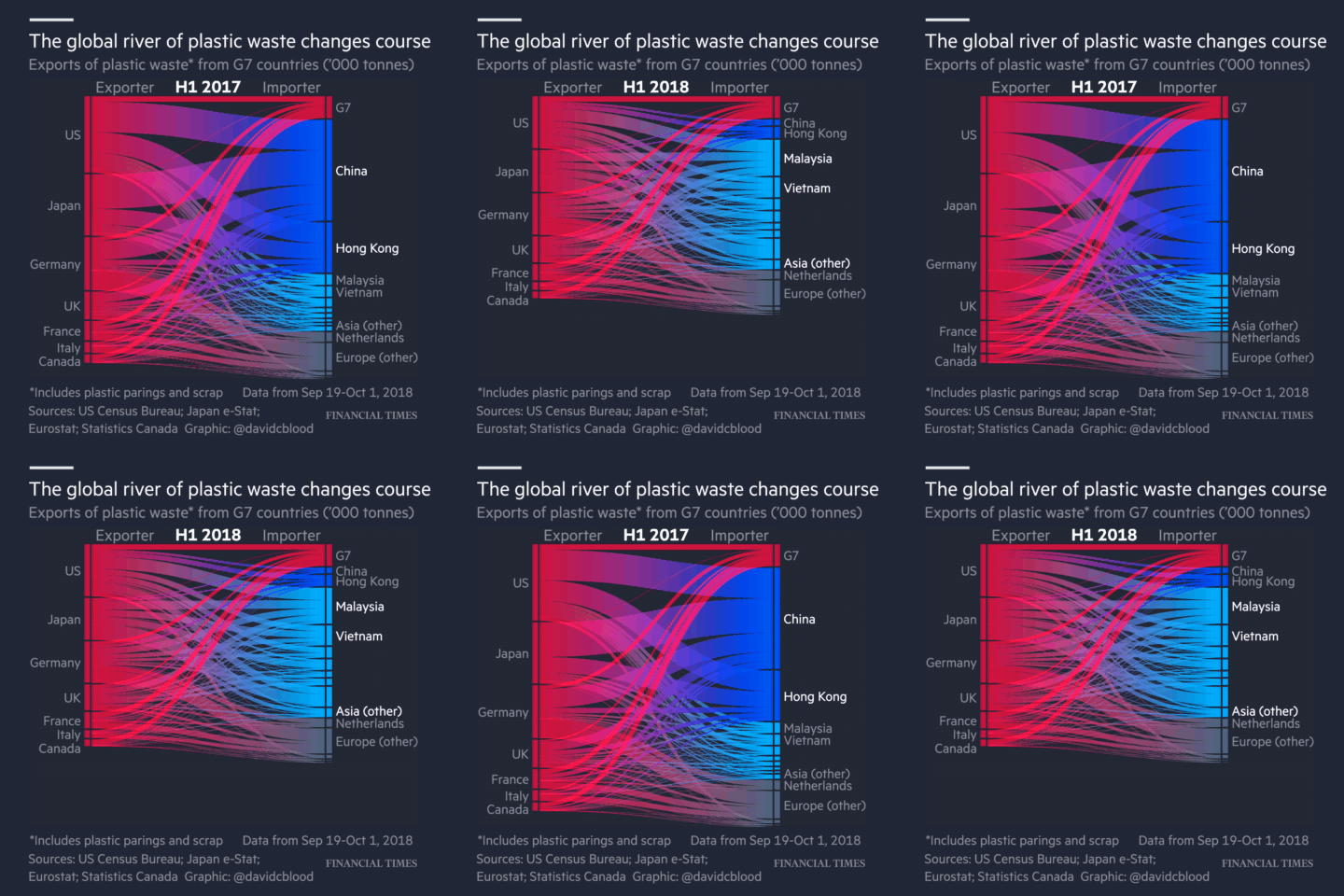
Animation from Financial Times article "Why the world's recycling system stopped working".

Those calculi try to capture the most interesting aspect of the programming language. This is function application in functional programming, sending of messages in concurrent programming and object construction with inheritance in object-oriented programming.

Recently, I have been working on programming tools for data exploration. In particular, I'm interested in the kind of programming that journalists need to do when they work with data. A good example is the coding done for the Why the world's recycling system stopped working article by Financial Times, which is available on GitHub.

Although data journalists and other data scientists use regular programming languages like Python, the kind of code they write is very different from the kind of code you need to write when building a library or a web application in Python.

In a paper Foundations of a live data exploration environment that was published in February 2020 in the open access Programming Journal, I wanted to talk about some interesting work that I've been doing on live previews in The Gamma. For this, I needed a small model of my programming language.

In the end the most interesting aspect of the paper is the definition of the data exploration calculus, a small programming language that captures the kind of code that data scientists write to explore data. This looks quite different from, say, a λ-calculus and π-calculus. It should be interesting not only if you're planning to do theoretical programming language research about data scripting, but also because it captures some of the atypical properties of the programs that data scientists write...

The Gamma: A language for simple data exploration

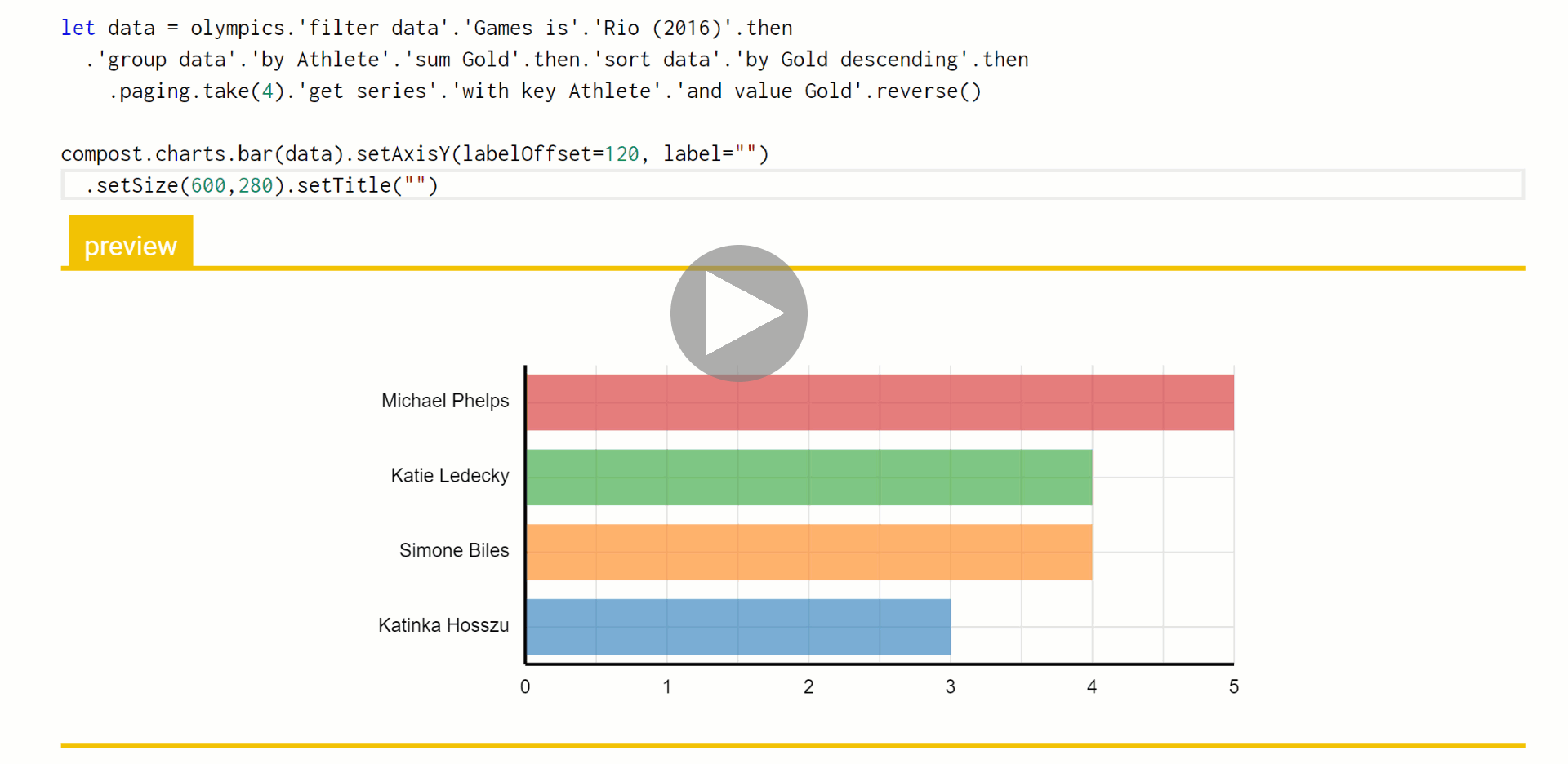
Before talking about the data exploration calculus and its interesting properties, I want to show you a few examples of the kind of data exploration scripts that I'm writing about. I will use The Gamma, a simple programming language for data exploration that I created, which uses type providers for accessing external data. The Gamma is simple, but you can create some non-trivial data visualizations like find who is the most frequent enemy of The Doctor using the Neo4j graph database as a back-end, or find out Michael Phelps compares to countries in the Olympics.

The following interactive playground shows a few of the examples from The Gamma gallery page. You can choose from a couple of pre-defined examples using the drop down. If you edit the code, click "Update page" to see the results.

The examples working with the Olympic medals is using a merged data set of Olympic games medals, which you can find on GitHub as a CSV file. It uses the pivot type provider which I described in a paper Data exploration through dot-driven development. As the name dot-driven suggests, The Gamma takes the idea of F# type providers to the extreme. The main way of using the environment is to start with an externally-defined value representing a data source such as olympics and type "." to see what members are available.

The pivot type provider uses the mechanism to let data analysts write simple SQL-like queries with grouping, filtering and sorting (but without joins). The other examples look at the World Bank data, which is a three dimensional data cube (with countries, years and indicators) and Dr Who graph database.

What kind of code data analysts write?

To understand what kind of code data analysts need to write when exploring data, have a look at the Jupyter notebooks in the GitHub repository for the Recycling is broken article. For example, the code from the notebook that wrangles the UN Comtrade data contains the following code. I removed some parts of the code (and used // for comments to make my syntax highlighter happy), but it is fairly representative:

 1: 
 2: 
 3: 
 4: 
 5: 
 6: 
 7: 
 8: 
 9: 
10: 

import pandas as pd

material = 'plastics' // 'plastics', 'paper'
df = pd.read_csv(
        f'data/raw/un-comtrade/{material}-exports-2017.csv',
        usecols=[3, 8, 9, 29], parse_dates=['Period Desc.']
    ) \
    .fillna(0) \
    .sort_values(['country_name', 'period']) \
    .reset_index(drop=True)

1: 
2: 
3: 
4: 
5: 
6: 
7: 
8: 

df_iso = pd.read_excel(
        'data/raw/Comtrade Country Code and ISO list.xlsx',
        usecols=[0, 1, 4, 7], na_values='N/A',
        keep_default_na=False // Necessary: The ISO2 code for Namibia is ‘NA’
    ) \
    .query('end_valid_year == "Now"') \
    .drop('end_valid_year', axis=1).dropna() \
    .reset_index(drop=True)

The code has a number of interesting properties:

• There is no abstraction. The data analysis uses lambda functions as arguments to library calls, but it does not define any custom functions. Code is parameterized by having a global variable material that is initially set to "plastics". Other possible values are stored in a comment. This works because there are only a few possible values. It also means that you can run individual code blocks in a Jupyter notebook and see the inline results, which would not work with a function.

• The code relies on external libraries. This analysis uses the Pandas library, which provides operations for data wrangling such as merge to join datasets or drop_duplicates to delete rows with duplicate column values. Such standard libraries are external to the data analysis and are often (in part) implemented in another language like C++.

• The code is structured as a sequence of commands. Some commands define a variable, either by loading data, or by transforming data loaded previously. Even in Python, data is often treated as immutable. Other commands produce an output that is displayed in the notebook.

• There are many corner cases. For example, the code sets the keep_default_na to False in order to handle Namibia correctly. Corner cases like this are typically discovered interactively by running the code and examining the output.

Introducing the data exploration calculus

The data exploration calculus aims to capture the first three observations. All interesting functionality is defined by external libraries and so the calculus itself is not Turing complete. The calculus combines functional features like lambda functions with object-oriented features like method calls. This is inspired by the earlier example of the Pandas data frame library.

Syntax of the data exploration calculus

The first thing we need to define is the syntax of the calculus. Objects \(o\) are defined by external libraries and have members \(m\), which can be invoked via dot. The syntax captures two of the above observations. First, a program \(p\) is formed by a sequence of commands \(c\). Second, lambda function can only be used directly as an argument to a method, but not assigned to a variable using \(\textbf{let}\) binding:

\[\begin{array}{rlcl} \textit{(programs)}\quad& p &::=& c_1; \ldots; c_n\\ \textit{(commands)}\quad& c &::=& \textbf{let}~x = t ~|~ t\\ \textit{(expressions)}\quad& e &::=& t ~|~ \lambda x\rightarrow e\\ \textit{(terms)}\quad& t &::=& o ~|~ x ~|~ t.m(e, \ldots, e)\\ \textit{(values)}\quad& v &::=& o ~|~ \lambda x\rightarrow e\\ \end{array}\]

Programs and commands are quite straightforward. A program is a list of commands separated by semicolons; a command is either \(\textbf{let}\) binding that assigns a term \(t\) to a variable \(x\) or a term \(t\) to be evaluated. The calculus distinguishes between terms and expressions. This is used to restrict how lambda functions can be used. An expression \(e\) can be a term or a lambda function whereas a term \(t\) can only be an object value, variable or a method call. Expressions (including lambda functions) can be used as arguments of a method call, but you can only assign terms (i.e. no lambda functions) to variables in \(\textbf{let}\) bindings.

How data exploration scripts evaluate

Now that we have the syntax of the data exploration calculus, we need to specify how programs in this language evaluate. The paper contains a formal definition of the reduction rules that define evaluation. The key thing is that the evaluation is defined using two relations:

\[\begin{array}{l} \rightsquigarrow & \quad \textit{(program evaluation)} \\ \rightsquigarrow_\epsilon & \quad \textit{(external library evaluation)} \end{array}\]

I'll illustrate what these mean using an example. Let's say that we have an external library for working with lists and for simple mathematical operations. The library defines two objects, \(\text{list}\) and \(\text{math}\) with some methods. You can think of those as global variables. It also defines list objects, which can be written as \([1,2,3]\). A list object also has some methods, including \(\text{map}\) and \(\text{sum}\). Here is a simple data exploration calculus program that uses these:

\[\begin{array}{l} \textbf{let}~l = \text{list}.\!\text{range}(0, 3)\\ l.\!\text{map}(\lambda x \rightarrow \text{math}.\!\text{mul}(x, 2)).\!\text{sum}() \end{array}\]

Programs evaluate from top to bottom, so start with \(\text{list}.\!\text{range}(0, 3)\). This is a method invocation and the way it evaluates is defined by the external library. In the formalism, this is defined by a relation \(\rightsquigarrow_\epsilon\). The relation is a part of the external library definition and the calculus uses it to evaluate method calls. In this case, the relation defines that \(\text{list}.\!\text{range}(0, 3) \rightsquigarrow_\epsilon [0, 1, 2, 3]\). After one step of the evaluation, we get:

\[\begin{array}{l} \textbf{let}~l = [ 0, 1, 2, 3 ]\\ l.\!\text{map}(\lambda x \rightarrow \text{math}.\!\text{mul}(x, 2)).\!\text{sum}() \end{array}\]

The next rule in the data exploration calculus specifies that, once a variable is reduced to a value \(v\), the value is substituted for the references to the variable. The object \([ 0, 1, 2, 3 ]\) is a value and so we get:

\[\begin{array}{l} [ 0, 1, 2, 3 ].\!\text{map}(\lambda x \rightarrow \text{math}.\!\text{mul}(x, 2)).\!\text{sum}() \end{array}\]

Now we have a chain of method calls and so we proceed from the left to the right. We start with the \(\text{map}\) operation. The argument of the operation is a lambda function. The relation \(\rightsquigarrow_\epsilon\), which defines the evaluation of external libraries, can be defined in terms of the main evaluation relation \(\rightsquigarrow\). In this case, it evaluates the function body for all the values in the list. The evaluation of those, in turn, again uses \(\rightsquigarrow_\epsilon\) to evaluate the \(\text{mul}\) operation:

\[\begin{array}{c} \text{math}.\!\text{mul}(0, 2) \rightsquigarrow 0,~~ \text{math}.\!\text{mul}(1, 2) \rightsquigarrow 2, ~\ldots~, \text{math}.\!\text{mul}(3, 2) \rightsquigarrow 6 \end{array} \]

The definition of \(\text{map}\) collects the resulting numbers and evaluates to a list \([ 0, 2, 4, 6 ]\). Now we just need one last step. Using the external library evaluation to evaluate the \(\text{sum}\) method, we get the result:

\[\begin{array}{l} [ 0, 2, 4, 6 ].\!\text{sum}() \rightsquigarrow 12 \end{array}\]

As you can see, the data exploration calculus has some familiar features like top-to-bottom evaluation and the use of substitution. However, there are a few aspects that are motivated by the nature of data scripting. Most actual computation is done by external libraries, which define the \(\rightsquigarrow_\epsilon\) evaluation relation. The calculus also does not specify how lambda functions evaluate - it is up to the external library to do this. Although, the definition in the paper specifies a few constraints to make sure that the library is reasonably behaved.

Using the data exploration calculus

One of the roles that formalisms like the π-calculus have is that they capture our understanding of certain types of programs in a way that programming language theoreticians (and a few other people who learn how to read the notation!) can understand. This alone is a valuable aspect. They make explicit the assumptions about what matters (at least to a theoretician) in a certain programming style.

However, the formalisms are also typically used for talking about other ideas. For example, you can use the λ-calculus to talk about various issues in type systems that may make it unsafe. You can also talk about various interesting extensions - how would, say, resource tracking interact with lambda abstraction?

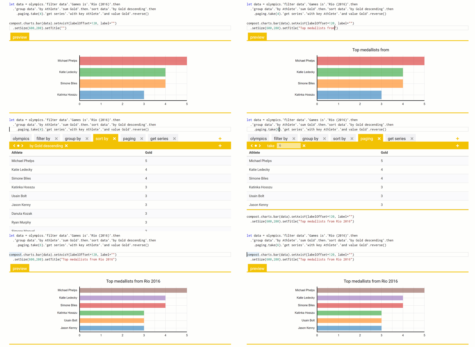
In Foundations of a live data exploration environment, I'm using the data exploration calculus to talk about an efficient way of evaluating live previews during code editing. This formalizes a mechanism that is actually implemented in The Gamma and you can play with it in the playground. Here is a little example where I use the pivot type provider to query a table with Olympic medals, add title to a chart and then modify the number of selected top results:

The important thing here is that the code to query the data source does not need to be re-evaluated each time an edit to the chart title is made. Furthermore, when I change the number of top results from 4 to 6, we still do not need to recompute the grouping and sorting of data. Using the data exploration calculus as my formalism, I can explain in a few pages how the mechanism works and prove certain properties about it - most importantly, the fact that the results it gives are the same as the results you'd get if you just evaluated the program from scratch each time an edit is made.

Conclusions

One aim of this blog post is to get more people who work on programming languages think about the kind of programming that is done when non-programmers like journalists explore data using, for example, a simple subset of Python with libraries like pandas. I think this is an interesting and important kind of programming that we should think more about!

One reason why I find data scripting interesting is that it lets us question many traditional assumptions about programming and programming languages. Consequently, we may get a fresh look at some standard issues. The data exploration calculus that I introduced in the Foundations of a live data exploration environment paper is one example. It blatantly breaks some typical rules: it is not Turing-complete and it does not have a mechanism for abstraction! Yet, it is enough to do some interesting data processing.

In the aforementioned paper, I use the calculus to talk about live previews. However, I imagine that there are many other interesting uses of the formalism and also many interesting extensions. Hopefully, this blog post will inspire you to explore some of them!